Forum Geografi, 31(2), 2017; DOI: 10.23917/forgeo.v31i2.4189

 

Analysis of Long-Term Temperature Trend as an Urban Climate Change Indicator

 

Dadang Subarna

 

Center for Atmospheric Science and Technology (LAPAN)

Jl. Dr. Djundjunan 133 Bandung, West Java

 

Corresponding Author (e-mail: dadang.subarna@lapan.go.id)

 

Abstract

Temperature plays a major role in detecting climate change brought about by urbanisation and industrialisation. Most climatic impact studies rely on changes in the average values of meteorological variables such as temperature. This paper attempts to study the temporal changes in the mean value of the air surface temperature over Jakarta city during the last century, specifically in the period 1901–2002.The data used in this study were taken from the Jakarta Climatology Station because they are of are good quality, there are extensive records and there is little missing or blank data. Statistic descriptive methods were employed, including a description of the type of probabilistic model chosen to represent the monthly mean air surface temperature time series. The long-term change in temperature was evaluated using the Mann-Kendall trend test method and the statistical linear trend test; the results of these two tests agreed. During the last 100 years, data observations from the station indicate that the monthly mean value of the air surface temperature of Jakarta city has increased at a rate of about 0.152°C decade^–1 and has not exhibited variability signals but has changed on average. Based on the linear regression model, the mean value of the air surface temperature over Jakarta city is estimated to reach around 28.5°C in 2050 and 29.23°C in 2100.

 

Keywords: Variability, Air Surface Temperature, Trend, Mann-Kendall, Climate Change.

 

Abstrak

Variabel meteorologi memainkan peranan penting dalam mendeteksi perubahan iklim yang disebabkan oleh urbanisasi dan industrialisasi. Kebanyakan studi tentang dampak iklim berdasarkan perubahan pada rata-rata variabel meteorologi seperti temperatur. Makalah ini mengkaji perubahan temporal pada rata-rata bulanan temperatur dan curah hujan di Kota Jakarta selama satu abad terakhir dengan periode 1901–2007. Data yang digunakan berasal dari Stasiun Klimatogi Jakarta yang relatif berkualitas bagus, rekaman berlangsung lama dan sedikit data hilang atau kosong. Metode yang dipakai adalah statistik deskriptik termasuk pemilihan tipe model probabilistik untuk menggambarkan rata-rata bulanan deret waktu temperatur. Perubahan temperatur jangka panjang telah dievaluasi dengan uji kecenderungan Mann-Kendall dan statistik regresi linear. Hasil uji kecenderungan Mann-Kendall sesuai dengan uji kecenderungan statistik regresi linear untuk data temperatur namun gagal mendeteksi untuk data curah hujan. Selama 100 tahun terakhir, data pengamatan stasiun menunjukkan telah terjadi kenaikan rata-rata bulanan temperatur udara Kota Jakarta dengan laju 0.152°C per dekade dan bukan tanda-tanda variabilitas semata. Didasarkan pada model regresi linear, maka temperaturpermukaan bulanan Kota Jakarta diperkirakan berada pada nilai 28.5°C pada 2050 dan 29.23°C pada 2100.

 

1. Introduction

It is not possible to predict when and where climate change will occur because of the uncertainty involved. Currently, scientists agree that global warming has occurred, even though it is still a debatable issue at the political level and among society (Gurevish et al., 2011). It is widely known that the air in the Antarctic is warming more rapidly than in the rest of the world and that the Antarctic Peninsula has experienced the greatest warming over the last 50 years (Hughes et al., 2006). The impact of climate change is characterised by the global warming trend. Temperature measurements taken using instruments around the world, both on land and on sea, have shown that, over the last 100 years, the earth's surface and the bottom part of the atmosphere has warmed by an average of 0.6°C (Buchdahl, 2002).

By using different climate models, various scientists have claimed that the earth's climate is currently unstable and that human activities play an important role in climate change. Rapid development and population growth has led to an ecological crisis around the world with varying degrees of damage. During the last century, climate change has had a great influence on the natural ecosystem and social economy aspect; for this reason, research into temperature changes is becoming very important and more and more studies are being carried out (Li, 2009). As a result of industrialisation and deforestation, the level of greenhouse gas (GHG) emissions has increased dramatically and changed the air composition of the atmosphere. Over the last 100 years, man-made GHG emissions, such as carbon dioxide, methane, and nitrous oxide, have increased; these three major gases resulted from the burning of fossil fuels and changes in land use (IPCC, 2008). In the last 20 years, it has begun to be assumed that these two phenomena are related to one another. In other words, the cause of the increase in the global average temperature is likely to be considered to also be a cause of the rise of GHG emissions, which have occurred simultaneously with the increasing concentrations of GHGs in the atmosphere.

According to the Intergovernmental Panel on Climate Change (IPCC) in 2008, the value and timing of climate change caused by all forms of both human and natural activities depend on the final concentration of the GHGs, aerosols, and their growth rates, as well as the response of the climate system in detail. GHG (especially CO₂) concentrations have increased significantly since the industrial revolution. The main impact of the increase in GHGs on the environment is that it causes global warming, which physically affects the absorption of short-wave radiation from the sun and suppresses long-wave radiation from the earth.

Other gases in the atmosphere, such as dust, particulates, smoke, and aerosols generated by human and natural activities, can obstruct solar radiation towards the earth that causes the cooling process in the earth's climate system. Nearly a third of the solar radiation received by the earth is reflected back into the atmosphere, while the rest is absorbed. Positive radiative forcing tends to warm up the earth's surface temperature, whereas negative radiative forcing tends to cool it down. In order to observe these radiation changes throughout the year, a study about air surface temperature needs to be conducted; the results of such a study would form basic knowledge of various climate change scenarios. A global climate change entails that regional climates also change (WMO, 2013). Studies related to climate variability determination, trends or fluctuations of temperature in the atmosphere are still rare in Indonesia. However, Subarna (2010) has used global data with 0.5°x0.5° grid data and validated these with some climatological station data to study the trends in spatial and temporal temperature in Indonesia. Irwansyah (2016) examined a sample of one year period in a study and suggested to investigate the climate change coverage over a longer period. Furthermore, it is also important to trace the changing because the effects of climate change start to appear in Indonesia.

Climate change will impact many aspects of livelihood, including its economy, poor populace, human health, and the environment (Measey, 2010). It also affects to the environment including precipitation, evaporation, run-off water and soil moisture; hence agricultural sector and food security will be affected (PEACE, 2007). Moreover, the effect of climate change on the ocean should also be regarded, especially for Indonesia as archipelagic island country. Increasing trend of sea level rise, warmer ocean temperature and increased of significant wave height are among a few example of climate change effects on the ocean that may affect to Indonesia (Zikra et al., 2014). The challenge for Indonesia is to create appropriate and effective adaptation strategies to address climate change and its impacts on building resilience and resistance. Hence the action needs to take place at all levels; from international, to national, to local and community-based efforts (Case et al., 2007)

Jakarta is one of the fastest growing cities in Indonesia that highly vulnerable to climate change effects. Aside from being the state capital, and therefore the administrative centre, it also is the centre of business and economy. For these reasons, the urbanisation occurring in various parts of the country will continue to increase in the future. As estimated by the World Bank (2002) in Dhorde et al. (2009), in a poor country as much as 80% of economic growth will emerge in the cities, and more than 80% of the world’s population will live in cities by the end of 2030. There is no doubt that cities will play an important role in shaping the economic value of developing countries. Cities are also currently (and will in the future be) facing many problems related to infrastructure and environmental damage.

The main concern relates to GHG emissions as a threat to the local and global climate regime. Several studies have shown that the increase in air surface temperature overwhelmingly occurred in urban areas as a result of urbanisation and population growth (Dhorde et al., 2009). According to the latest estimation from the IPCC in 2007, the earth’s surface average temperature has increased linearly by 0.74°C during the period 1901–2005. The investigation related to the impact of urbanisation and land use changes toward the surface temperature average is considered as a very important study.

Air surface temperatures are associated closely with human activities. These temperatures have a great daily variability and are easily influenced by local topography effects (Hasler et al., 2015). Total transformation of the natural landscape into housing, roads, fields, large buildings and industrial installations has changed the climate on a regional basis in the big cities (Carter et al., 2015). The main reasons for the difference in temperatures of various cities are the heat balance and water balance (Ming et al., 2014). These are affected by the transformation of the earth’s surface into concrete and asphalt, causing a quick dry off precipitation (Shahmohamadi et al., 2011). Other causes include the surface roughness which has increased due to the construction of buildings, the heat supplied by the domestic industries, and vehicle traffic and other forms of combustion that aggravate the air quality in the city (Carter et al., 2015). The purpose of this research is to study the monthly average of the air surface temperature in Jakarta during the last century and to analyse how the local and regional temperature has changed; this constitutes one of the simplest indicators to prove the occurrence of climate change.

2. Research Method

The average air surface temperature data for the period 1901–2002 used in this paper were obtained from the Jakarta Meteorology, Climatology and Geophysics station (BMKG), and are shown in Table 1 and Figure 1. The air temperature measured by the thermometer is an essential climate element as it affects the life of the biosphere greatly. An air temperature measurement only produces one value which states the average value of the air temperature.

 

Table 1. WMO Code and description of Jakarta station of Meteorology

Country	WMO Code	City	Elevation	Latitude	Longitude	Period
515	9674500	Jakarta/Observatory	-	−6.18	106.83	1901–2002

 

Temperature can also be defined as the heat level of an object. Heat moves from an object with a higher temperature to objects with lower temperature. Air temperature changes according to time and place. In general, the maximum temperature occurred after noon, usually between 12:00 and 14:00, and the minimum temperature occurred at 06:00 or around sunrise. The daily air temperature average is defined as the average value from a 24-hour observation (one day) with measurements being taken every hour. The average monthly temperature is the sum of the average daily temperatures in one month divided by the number of days in the month; this method is used in the statistical analysis in this paper.

Figure 1. Air surface temperature average during 1901-2002 in Jakarta Meteo station

The methods used in this research are summarised by the diagram in Figure 2. The quality and consistency of the data has been checked and polynomial interpolation has been performed in order to fill in the missing data or empty data using Minitab. Data consistency was obtained by calculating the coefficient of variability. Statistical data characteristics are displayed with a summary of the data description and the approach of the probability density function (PDF).

Figure 2. Schematic flowchart of temperature data time series

To test the increase or decrease tendency (trend) of the data, the non-parametric statistical test devised by Mann-Kendall was used (Onoz et al., 2003). The Mann-Kendall test is based on S statistics. Each pair of the observed value yi, yj (i>j) of the random variable is checked to find either yi>yj or yi<yj. If the number of the previous pair was P and the number of the next pair is M, then S is defined as S=P−M. For n>10, the distribution of samples of S is defined as Z. Whereas Z follows the standard normal distribution as described by Equation 1.

                                (1)

where,

 

The null hypothesis is rejected when the calculated value of Z is greater than the absolute values of Z_{α/ 2}. The Mann-Kendall test is often used as the non-parametric test since it has the ability to detect the slope tendency (trend), sample size, significant level, coefficient of variation, and type of probabilistic distribution. These capabilities are not possessed by the usual linear statistical test. The approach used in this study is that the assumption of temperature satisfies the normal probability distribution function. The normal probability distribution is one that describes the distribution of the random variable which often appears in real life. Random variables such as temperature, for example, x, will follow the normal distribution if the PDF satisfies the Equation 2.

                  (2)

where μ is the average and σ is the standard deviation.

The LST (Land Surface Temperature) has also been derived from the Aqua satellite in order to evaluate the spatial distribution of temperature in the last decade. The Aqua satellite platform has the MODIS (Moderate Resolution Imaging Spectroradiometer) sensor on board, which acquires the LST data. MODIS data is disseminated via LAPAN’s website (http://bisma.sains.lapan.go.id/), from which the LST data for this research can be downloaded. These data can be processed using the Python scripts (see Appendix 1). The MODIS sensor detects emitted and reflected radiance in 36 channels spanning the visible to infrared (IR) spectrum. Further information about the instrument can be found on the NASA MODIS website (http://modis.gsfc.nasa.gov/about/specifications.php). The electromagnetic radiation emitted from the sea surface can be inverted using Planck’s law to deduce the surface temperature of the target. For remote sensing applications, the 11–12 μm spectral window is used most frequently because of its relatively low sensibility to the earth’s atmosphere (Morales et al., 2011). The nominal image resolution of the data (at the satellite nadir) is 1 km and its effective radiometric resolution for LST is 0.1°C.

3. Results and Discussion

To achieve the research objectives, the temperature time series data during the last 100 years have been analysed in terms of its variability, patterns and statistical measures. Variability of air surface temperature in Jakarta is indicated by the variability coefficient of 0.0264 or 2.6%. The variability coefficient is very small, which means that the temperature consistency is very high. These results indicate that the variations did not fluctuate sharply and were relatively close to the deviation of the average condition meaning that the monthly average air surface temperature in Jakarta is relatively stable. From the temperature data, the descriptive statistics and its probability functions are defined. Descriptive statistics of the monthly temperature data in Jakarta are summarised in Table 2. There were several values which required extra attention: variance, skew, and kurtosis. Variance is a measure of how far the temperature data spreads from its mean value, and can be calculated by averaging the square of the difference to the mean value.

 

Table 2. Descriptive statistics of the monthly average of air surface temperature data in Jakarta

Statistics	Temperature data description
Amount of data	1224
Maximum value	29.2
Located in line	1223
Minimum value	24.3
Located in line	207
Mean value	26.9
Mean deviation value	0.6
Standard deviation	0.7
Variance	0.5
Skew	0.07
Kurtosis	−0.00927

 

In Table 2 it is shown that there was only one negative value, that of kurtosis (−0.00927). Kurtosis is a measure that indicates whether the probability function is oval in shape or flat, relative to the normal distribution form. The lower negative kurtosis value means that the temperature probability function around Jakarta is slightly flatter than the normal distribution, as shown in Figure 3. The skew value was approximately 0.074, which means that the symmetrical temperature distribution form is proportional to the left and right of the average value. The probability distribution function (Equation 2) also shows that the temperature data have a balanced probability density which spreads to the left and right of the mean value of 26.94°C. The normal probability distribution and the normal curve are often referred to as Gauss distributions and curves.

Figure 3. The probability density function of temperature and its comparison with the normal distribution function

This distribution is one of the most important and widely used. The normal probability distribution is strongly influenced by the mean temperature value (μ) of 26.94°C and the standard deviation value (σ) of 0.711°C. The higher the standard deviation values, the more declivous the curve becomes; on the other hand, the smaller the standard deviation values, the more pointed the curve. Comparing the average values with the standard deviation values showed a significant difference; therefore, the temperature probability density curve was characterised by a having a slightly tapered upward peak and may be classified as leptokurtic. This smaller value of standard deviation indicates that temperature data are grouping at the average value or median value.

Trend analysis was carried out using a linear trend model performed on the whole temperature data. This linear regression model is a very simple way of predicting the data trend in the future. The results of the trend analysis, along with the linear equations and the accuracy of the model, are shown in Figure 4. The linear regression equation of temperature change over time was defined as Yt=26.1634+0.00126397*t with a gradient of 0.00126397°C. This value indicates that the monthly average value of air surface temperature in Jakarta has a tendency that continues to rise by 0.00126397°C per month. Assuming the gradient increases equally each month, then within ten years the rise in the city temperature will reach the value of 0.152°C. This result falls within the same range as the predicted values based on the analysis that has been undertaken by BMKG of cities in Indonesia, specifically, between 0.036°C and 1.383°C per ten years (KOMPAS, 2009).

Figure 4. Linear tendency analysis of air surface temperature in Jakarta

The accuracy of the linear trend model is indicated by the MAPE (Mean Absolute Percentage Error), MAD (Mean Absolute Deviation) and MSD (Mean Squared Deviation) values of 1.614, 0.4 and 0.30, respectively, which measure the accuracy of the time series value of the matched temperature. These values are small enough to indicate an acceptable level of accuracy. However, to eliminate doubt, another Mann-Kendall test was performed to check each piece of data over the before and after data, as shown in Equation 1. Each pair of observed data values yi, yj (i>j) of random variables were assessed to determine whether yi>yj or yi<yj. The Mann-Kendall test results are shown in Table 3.

 

Table 3. Mann-Kendall test results on the temperature time series data

Kendall's tau	0.461
S	337549.000
p-value (two-tailed)	< 0.0001
alpha	0.05

Null hypothesis H₀: There is no trend in the temperature time series

H₁: There is an irregularity in the temperature time series

 

If the p-value from the calculation is smaller than the alpha significance level of 0.05, then the null hypothesis H₀ will be rejected and the alternative hypothesis H₁ will be accepted. The consequences of the rejection of the null hypothesis H₀ are justified if the p-value is lower than 0.01%. From Table 3, we can see some test parameters of the Mann-Kendall tendency. There are three important S values in the test (see Equation 1). A large negative S value indicates a downtrend and a large positive S value indicates an upward trend, whereas a zero value indicates no inclination. The Mann-Kendall temperature tendency test has a very large S value, which means that it can be concluded, with a high confidence level, that there is a tendency of the temperature to rise. The null hypothesis H₀ should be rejected because the p-value from the calculation is 0.0001 smaller than the alpha significance level of 0.05; this is highly justified because it is lower than 0.01%. Statistical methods of decomposition and the multiplicative model with the formula (Yt = seasonal tendency * error) were used to separate time series data linear and seasonal tendencies and their error components; the results are shown in Figure 5.

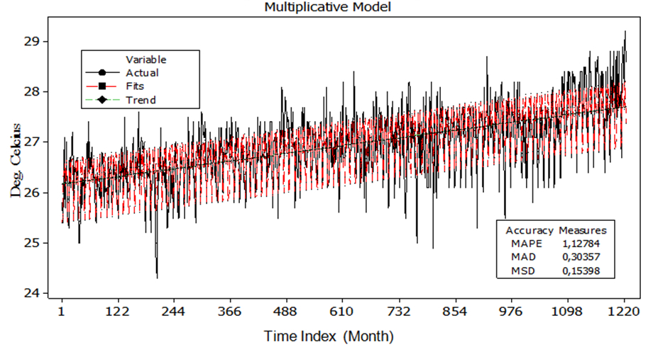
Figure 5. Multiplicative model and its original temperature data and the accuracy measurements

The multiplicative model is employed when the size of the seasonal pattern depends on the data level. This model assumes that, if the data increases, the seasonal pattern will also increase. In other words, this method demonstrates that the increase in temperature was not caused by the seasonal pattern, but the overall data experienced an increase on both the average and the seasonal level. From Figure 5, we can see the accuracy of the MAPE, MAD and MSD, respectively, at 1.13, 0.3 and 0.15. These values are small enough that the model is considered acceptable.

Figure 6. Average temperature movement every 30 years shift period.

Figure 6 shows the evolution of the average air surface temperature, which shifted every 30 years. The figure above provides evidence that the average temperature propagation in Jakarta has continued to rise over the last 100 years. The analysis is focused on the changing of the mean value every 30 years, and the century is divided into eight periods, as shown in Table 4. From Figure 6 and Table 4, it is clear that the temperature gradient shows a positive increase and it does not represent mere variability or a seasonal increase gradient.

 

Table 4. Temperature average every 30 years during 1901–2002

No	Periods	Temperature average (°C)
1	1901–1930	26.3
2	1910–1940	26.5
3	1920–1950	26.7
4	1930–1960	26.8
5	1940–800	26.8
6	1950–1980	26.9
7	1960–1990	27.1
8	800–2002	27.2

 

A relatively small gradient decrease occurred during the periods 1930–1960 and 1940–1970. This also occurs on the annual average of global surface air temperatures in 1880-2014 [(see Voiland (2011)]. Throughout the period of 1960s to 1970s, the average global temperature remained relatively cool. During the 1960s, weather experts found that over the past couple of decades the trend had shifted to cooling. In the early 1970s some scientists predicted a continued gradual cooling, perhaps a phase of a long natural cycle or perhaps caused by human pollution of the atmosphere (NASA, 2015). Meanwhile, a relatively large gradient increase occurred during the periods 1960–1990 and 1970–2002, which are the periods of rapid development in the economic and infrastructure sectors in Jakarta. If the analysis of the trend and its linear regression model assumes a scenario in which there will be no mitigation efforts or limitations of business development, then it is estimated that the average monthly air surface temperature in Jakarta will reach approximately 28.5°C in 2050 and 29.23°C in 2100. It means that the absolute percentage error is 1.614.

This increase in temperature, both on a global and a local scale, is expected to trigger changes in many aspects of the weather, such as wind patterns, convective potential energy, amount, type and frequency of rain and extreme weather events. As a widely known fact, it cannot be denied that the occurrence of extreme rain can cause floods, whirlwinds and small tornadoes (IPCC, 2013). These events will bring side effects in terms of environmental, social and economic issues and people will be particularly vulnerable if such events are not anticipated as early as possible.

The results of satellite image processing for LST of Jakarta city from the MODIS sensor currently on board the Aqua spacecraft are shown in Figure 7. From Table 4 and Figure 7, it can be seen that, in the last 30-year period, the monthly mean temperature has been around 27.2°C. Figure 7 shows the instantaneous LST in the dry season and in the transition from dry to wet. There are some hot spots which represent high temperatures of around 37°C. These can come from the transportation and industry sources. The combination of the urban heat island effect, as a local phenomenon, and climate change, as a global phenomenon, can bring higher temperatures to urban areas than their surrounding areas.

 

Figure 7. The land surface temperature (in °C) of Jakarta city in the last 30 years in the dry season (a) and in the transition from dry to wet (b), derived from the MODIS sensor on board the Aqua satellite

 

4. Conclusion and Recommendation

The monthly average air surface temperature data obtained from BMKG over a period of 101 years, from 1901 to 2002, has been processed and analysed using statistical methods. The probability distribution function of the air surface temperature data in Jakarta was found to be symmetrical – this means the probability is proportional to the left and to the right of the average value – and the temperature probability density curve is characterised by having a slightly tapered upward peak; in other words, the curve may be classified as leptokurtic. From the linear trend test, the linear regression equation of temperature changes over time was obtained and was defined as Yt=26.1634+0.00126397*t with a gradient of 0.00126397°C. This indicates that the monthly average air surface temperature in Jakarta has a tendency of a constant rise by 0.00126397°C per month. The accuracy of the linear trend model was indicated by the MAPE, MAD and MSD values of 1.614, 0.4 and 0.30, respectively; these values match the accuracy of the temperature time series value and are therefore acceptable.

The Mann-Kendall trend test of temperature data showed that there was a very large S value; this means that it can be concluded, with a high confidence level, that there is a rising tendency. Moreover, the null hypothesis H₀ must be rejected because the p-value from the calculation is 0.0001 smaller than the alpha significance level of 0.05; this condition is highly justified because it is less than 0.01%. If the gradient is assumed to increase constantly each month, then within ten years the temperature increase will reach 0.152°C.

This result falls within the range of values predicted based on the analysis that has been undertaken by BMKG of cities in Indonesia, specifically, between 0.036°C to 1.383°C per ten years. If the trend and its linear regression model assume that there will be no scenarios of mitigation and limitation of business development, then it is estimated that the monthly average air surface temperature in Jakarta will be around 28.5°C by 2050 and around 29.23°C by 2100. Pre-emptive action should be taken to limit temperature increase by multiplying and extending the city parks, reducing GHG emissions, building environmentally friendly urban infrastructure, and urban bioforestation, among other methods.

Acknowledgements

The author thanks to Centre for  Atmospheric  Science and Technology LAPAN for the financial  support  and  The Meteorology, Geophysics and Climatology Agency BMKG for data sharing.

References

Buchdahl, J. (2002). Weather and Climate Teaching Pack, www.ace.mmu.ac.uk Accessed on 12 Maret 2013

Carter, J.G., G. Cavan, A. Connelly, S. Guy, J. Handley and  A. Kazmierczak. (2015). Climate change and the city: Building capacity for urban adaptation. Progress in Planning, pp.1-66

Case, M., F. Ardiansyah  and  E. Spector. (2007). Climate Change in Indonesia: Implications for Humans and Nature. www.wwf.or.id . Accessed on 22 August 2017

Dhorde, A., A. Dhorde1, and A. S.Gadgil. (2009). Long-term Temperature Trends at Four Largest Cities of India during the Twentieth Century. J. Ind. Geophys. Union Vol.13, No.2, pp.85-97.

Gurevish, G., Y. Hadad. A. Ofir and B.Ohayon. (2011). Statistical  Analysis of Temperatur Change In Israel: An Application fF Change Point Detection and Estimation Techniques. Global NEST Journal, Vol 13, No 3, pp 215-228.

Hasler, A. , M. Geertsema , V. Foord1 , S. Gruber , and J. Noetzli. (2015). The influence of surface characteristics, topography and continentality on mountain permafrost in British Columbia The Cryosphere, 9, 1025–1038

Hughes, G. L., S.S. Rao and T.S. Rao. (2006). Statistical analysis and time-series models for minimum/maximum temperatures in the Antarctic Peninsula. Proc. R. Soc. A.

Irwansyah. (2016). What do scientists say on climate change? A study of Indonesian newspapers. Pacific Science Review B: Humanities and Social Sciences 2 58-65

IPCC. (2008). Working Group II IPCC Fourth Assessment Report, Working Group II Report "Impacts, Adaptation and Vulnerability", Chapter 3, Freshwater Resources and their Management, tersedia pada http://www.ipcc.ch/ipccreports/ar4-wg2.htm. Accessed on 28 Desember 2012

IPCC. (2013). Climate Change. The Physical Science Basis. Contribution of Working Group  I to the Fifth Assessment Report of the IPCC. Summary for Policymakers are available from the IPCC website www.ipcc.ch and the IPCC WGI AR5 website www.climatechange2013.org

KOMPAS. (2009). Suhu Udara di Indonesia Rata-rata Naik: Kenaikan di Beberapa Kota di Atas Satu Derajat Celsius, KOMPAS GRAMEDIA, Terbitan 31 Maret 2009

Li, X. (2009). Applying GLM Model and ARIMA Model to the Analysis Of Monthly Temperature of Stockholm. D-level Essay in Statistics in Spring 2009 Department of Economics and Society, Dalarna University

Measey, M (2010). Indonesia: A Vulnerable Country in the Face of Climate Change. Global Majority E-Journal, Vol. 1, No. 1, pp. 31-45

Ming, T., R.  de_Richter, W. Liu  and S. Caillol. (2014). Fighting global warming by climate engineering: Is the Earth radiation management and the solar radiation management any option for fighting climate change?. Renewable and Sustainable Energy Reviews V. 31,  pp. 792–834

Morales J., V. Stuart, T. Platt and S. Sathyendranath. (2011). Handbook of Satellite Remote Sensing Image Interpretation: Applications Marine  for Living Resources Conservation and Management. The EU PRESPO Project and IOCCG

Zikra , M., Suntoyo and Lukijanto. (2015). Climate change impacts on Indonesian coastal areas. Procedia Earth and Planetary Science 14, 57 – 63

NASA. (2015). World of Change: Global Temperatures. https://earthobservatory.nasa.gov/NaturalHazards/.accessed  at  6 August 2017

PEACE. (2007). Indonesia and Climate Change: Current Status and Policies World Bank

Onoz, B., and M. Bayazit. (2003). The Power of Statistical Tests for Trend Detection, J. Eng. Env.Sci. Vol.27, 247-251, TUBITAK Turkish

Subarna, D. (2010). Analisis Variabilitas Suhu Permukaan Bulanan di Atas Kepulauan Indonesia Selama Satu Abad Terakhir. Prosiding Seminar Nasional Sains Atmosfer I 2010, Bandung 16 Juni 2010, 142-147 

Shahmohamadi, P., A. I. Che-Ani, K. N. A. Maulud, N. M. Tawil, and N. A. G. Abdullah. (2011). The Impact of Anthropogenic Heat on Formation of Urban Heat Island and Energy Consumption Balance. Urban Studies Research, V.2011, Article ID 497524, p. 9

Voiland, A. (2011). Global temperature records in close agreement. Retrieved 6 December 2017, from https://climate.nasa.gov/news/468/global-temperature-records-in-close-agreement/

WMO. (2013). The Global Climate 2001–2010: a Decade of Climate Extremes Summary Report. WMO-No. 1119. CH-1211 Geneva 2, Switzerland

 

Appendix 1: Python Script for Satellite Image Processing

import os

import gdal

import gdalnumeric

import pylab

from mpl_toolkits.basemap import Basemap

import numpy as np

import matplotlib.pyplot as plt

folder_data = 'C:/Python32/Data'

folder_hasil = 'C:/Python32/Hasil'

os.chdir (folder_data)

files = os.listdir(folder_data)

for i in range (len(files)):

filename = files[i]

dataset = gdal.Open('C:/Python32/Data/t1.15274.0317.modlst.hdf')

list_dataset = dataset.GetMetadata('SUBDATASETS')

lat = gdalnumeric.LoadFile(list_dataset["SUBDATASET_1_NAME"])

lon = gdalnumeric.LoadFile(list_dataset["SUBDATASET_2_NAME"])

LST = gdalnumeric.LoadFile(list_dataset ["SUBDATASET_3_NAME"])

LST = 0.1000000015*(LST)

lat_min = -06.7

lat_max = -05.7

lon_min = 106.5

lon_max = 107.2

m = Basemap(projection='cyl',llcrnrlat=lat_min,\

urcrnrlat=lat_max,llcrnrlon=lon_min,urcrnrlon=lon_max,resolution='h')

m.drawcoastlines()

parallels = np.arange (-90,90,5)

m.drawparallels(parallels,labels=[1,0,0,0],fontsize=10)

meridians = np.arange (0,360,10)

m.drawmeridians (meridians,labels=[0,0,0,1],fontsize=10)

clevs = [21,22,23,24,25,26,27,28,29,30,31,32,33,34,35]

x,y = m (lon,lat)

cs = m.contourf(x,y,LST,clevs)

cbar = m.colorbar (cs,location='bottom',pad='10%',size='5%')

cbar.set_label ('Kelvin')

pylab.title ('Temperature_Permukaan(Kelvin) '+filename)

plt.savefig(folder_hasil+"/"+filename+".png");

plt.close();

 

 

© 2017 by the authors. Submitted for possible open access publication under the terms and conditions of the Creative Commons Attribution (CC-BY-NC-ND) license (http://creativecommons.org/licenses/by/4.0/).